
When detecting objects in images, the Histogram of Orientated Gradient (HOG) descriptor combined with a Linear Support Vector Machine (SVM) is one of most powerful techniques available. Despite more recent advances in neural-network based object detection, the HOG + Linear SVM combination remains an object detection workhorse for small to medium sized datasets. This article examines the underlying theory of the Support Vector Machine and explains how it can be applied to solve computer vision problems.
Large Margin Classification
To illustrate the workings of the SVM, we’ll first consider a non-computer vision Machine Learning problem with two classes and two features. For background on Machine Learning, refer to our Machine Learning introduction and Machine Learning model articles. In the image below we have two classes (gray and blue), described by two features (X1 and X2).
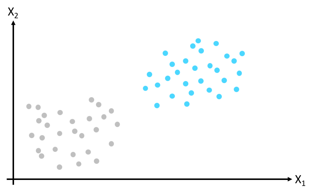
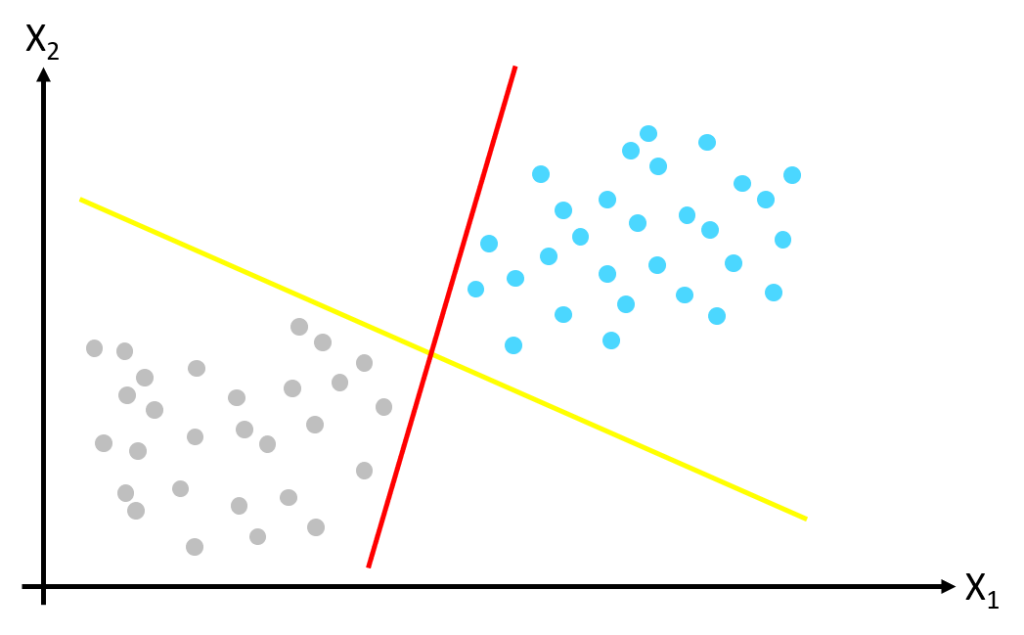
To create a Machine Learning model separating the classes above, the SVM simply finds a line that divides the classes. This line becomes a plane (also known as a manifold) when there are more than two dimensions i.e. more than two features describing the classes. In the image above, the two classes are linearly separable (they can be separated by a straight line) however, as the image below illustrates, there are many possible positions for the class separation boundary. Both the yellow and the red lines separate the training dataset but they will perform very differently when classifying new data instances.
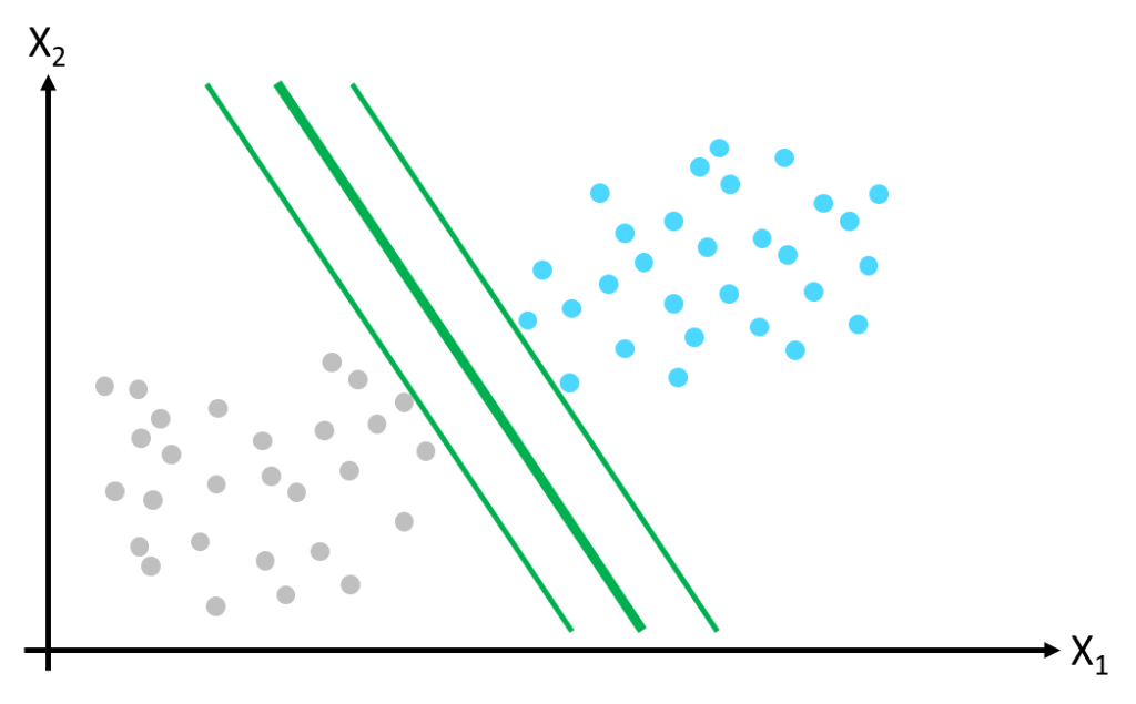
To find the best class separation boundary, the SVM performs large margin classification. Rather than drawing a zero-width line between classes, we fit a margin around the separating line and choose the line position which maximizes this margin. The thicker green line in the image below represents the class separation boundary.
Only a few of the training data points touch the edges of the margin – these are known as support vectors. Only the support vectors influence the position of the class separation boundary – adding more data points away from the margin has no influence on the class separation boundary.
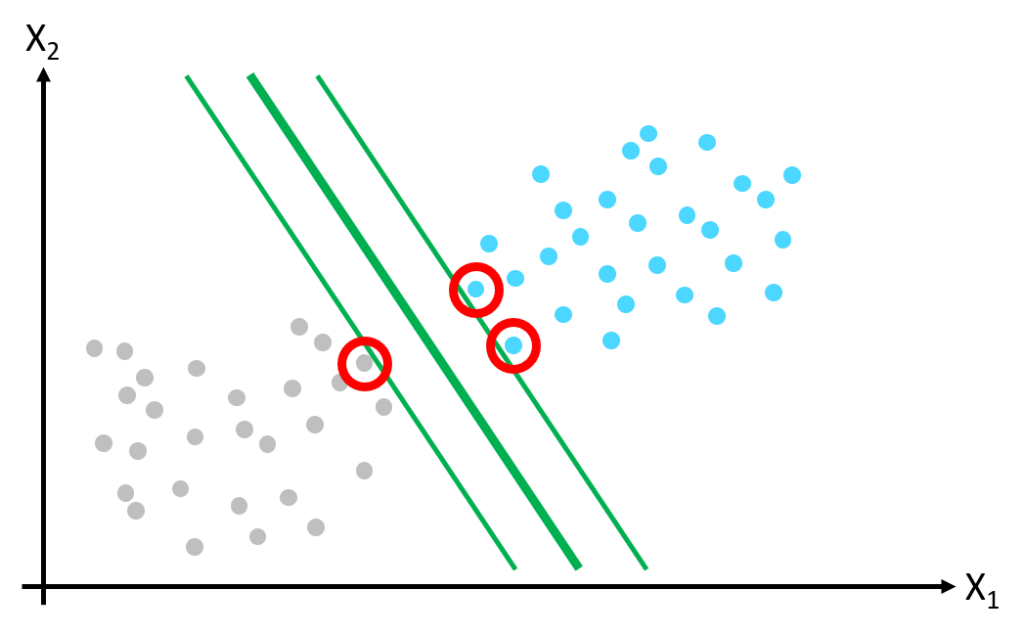
The advantage of separating the class boundary with very few data points (the support vectors) makes the SVM very computationally efficient, giving real-time inference of new data points. This approach however makes the SVM very sensitive to feature scales therefore it is vital to apply scaling to input data before fitting the SVM model.
Soft Margin Classification
Imposing that all training data points be outside of the margin is called hard margin classification. This approach only works if the data is linearly separable and has no outliers. A more flexible approach is required to manage these issues. The SVM model’s hyperparameter, known as the C value, controls the degree to which training data points are allowed to enter the margin. This technique is called soft margin classification. Reducing the C value results in a wider margin with more data points inside the margin.
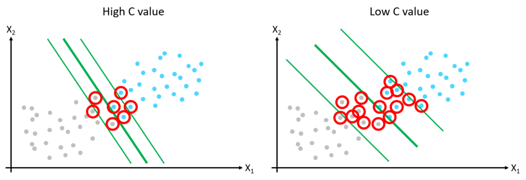
The C value is a simple but effective model hyperparameter. If a SVM model is overfitting the training data, this can be regularized by reducing the C value.
Applying the SVM in Computer Vision
The SVM is a conventional Machine Learning model i.e. it does not make use of Deep Learning neural network techniques. When working with images, conventional Machine Learning models operate with an intermediate representation of the image (or part of the image). This intermediate representation is generated by an image descriptor, for example a Histogram of Orientated Gradient (HOG) descriptor or a Haralick texture descriptor. When applied to an image, or a region of interest, an image descriptor converts raw pixel intensities to a feature vector. The length of the feature vector depends on the image descriptor used.
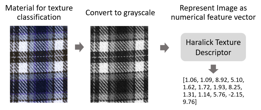
The illustrations in the first section of this article contain only two features (X1 and X2) to describe the classes. The Haralick texture descriptor applied in the illustration above outputs a vector of 13 features. Each of these 13 features becomes an input to our SVM classifier, giving a dataset of 13 dimensions.
To demonstrate this concept, consider a training dataset of images containing stop signs. The stop signs in the training data are manually annotated to identify the region of interest. The HOG descriptor takes the region of interest from each of the training images and generates a feature vector of real-valued numbers for each training image. When using HOG, the length of the feature vector depends on the HOG parameter settings. A SVM model is then trained on the HOG feature vectors, learning the HOG filter that represents a stop sign.
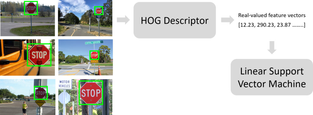
Having trained a SVM model on a number of annotated training images, a new image can be presented to the model which is thought to contain a stop sign. The HOG descriptor is slid over the new image at varying scales, extracting a feature vector at each point. The feature vectors are then presented one by one to the SVM model, which determines the presence of a stop sign based on the HOG filter learnt during the model training phase.
Conclusion
The Support Vector Machine remains the cornerstone of conventional Machine Learning. It’s a powerful model which can perform well on small, high-dimensional datasets. As oppose to neural networks, conventional Machine Learning models do not deal directly with raw pixel intensities but rather with an intermediate representation of the image or region of interest. The intermediate representation is in the form of a real-valued vector which is generated by an image descriptor. Many image descriptors are available, such as the Histogram of Orientated Gradient descriptor and Haralick texture descriptor.