
Image distortion can cause havoc with visual inspection systems if not correctly addressed. This article describes how to correct for distortion using OpenCV’s camera calibration functions.
Projective Geometry – the pinhole camera
The pinhole camera is an idealized model of a camera in which an imaginary wall with a tiny hole in the center blocks all rays of light except those passing through the aperture. As only a single ray enters the pinhole from any particular point in the scene, the resulting image on the projection (imager) surface is always in focus. The size of the projected image is governed by the distance between the imager surface and the aperture – this is the focal length of the camera.
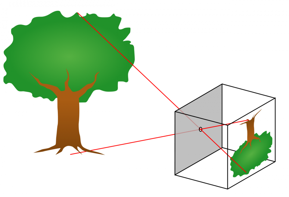
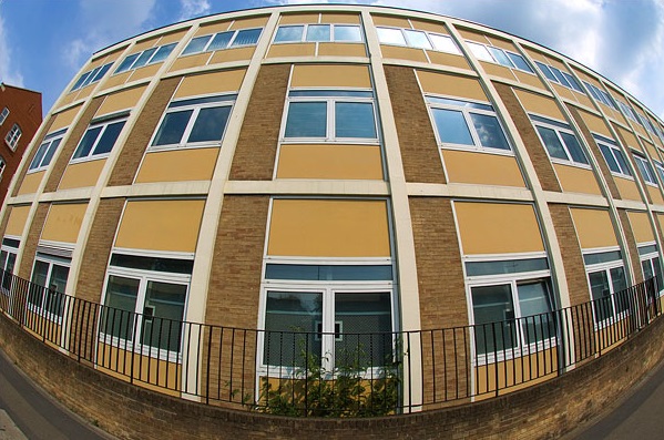
In practice, a pinhole camera doesn’t work because it cannot gather sufficient light for rapid exposure. This is why human eyes and cameras use lenses to gather more light. The downside of lenses is that they introduce distortion. The most common form of distortion is ‘barrel’ distortion, when straight lines are curved inwards in the shape of a barrel.
Camera calibration is the application of mathematical corrections to account for the deviations from the idealized pinhole camera model which are imposed by the use of a lens.
The camera intrinsics matrix
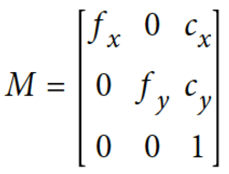
In order to project points in the physical world into the camera’s imager plane, the main piece of information needed is the focal length. We require two focal lengths, fx and fy, recognizing that individual pixels on an imager are not perfect squares and their rectangular nature must be taken into account. Secondly, the imager chip is usually not perfectly centered with the optical axis of the camera due to manufacturing tolerance limits. The values cx and cy represent the displacement of the imager center from the camera’s optical axis. These four values are combined into a 3 x 3 matrix known as the camera intrinsics matrix.
Lens distortion
In theory it is possible to define a lens that introduces no distortion. In practice, largely due to manufacturing reasons, it is difficult and expensive to produce such a lens. Furthermore, it is difficult to perfectly align the camera lens and the imager sensor.
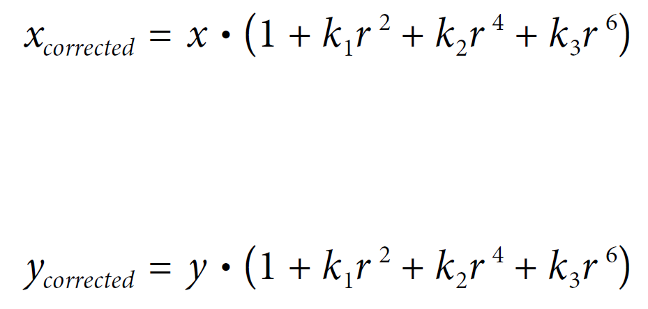
The two main types of distortion resulting from the lens are radial distortion and tangential distortion. Radial distortion arises from the shape of the lens whereas tangential distortion is caused by the assembly process of the camera. The bulging effect known as barrel or fish eye distortion is caused by radial distortion in the camera. Rays further from the center of the lens are bent more than those closer to the center of the lens hence the sides of a square appear to bow out. To correct for radial distortion, three coefficients are used: k1, k2 and k3. The x and y values are the original locations (on the camera imager) of the distorted points and the corrected values are the new locations as a result of correction.
To account for tangential distortion, we require two additional parameters: p1 and p2, giving a vector of five distortion parameters in total (k1, k2, k3, p1 and p2).
Camera calibration
Having defined the calibration model, we’ll now perform the calibration process using OpenCV. In order to determine the 9 parameters described above (4 camera intrinsics coefficients and 5 distortion coefficients), we need a number of distorted chess board images – a dataset of at least 10 images is recommended, taken with the camera to be calibrated.
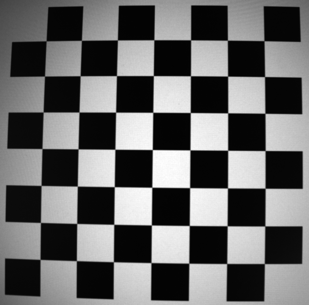
We start by making imports and setting up data for later use in the calibration process. A termination criterion is required for OpenCV’s cornerSubPix() function, which performs high accuracy searches for corners in chess board images. A set of object points is required to tell OpenCV that we are using an 8 x 8 chess board as our calibration target.
import cv2
import numpy as np
import glob

# setup termination criteria for cornerSubPix()
criteria = (cv2.TERM_CRITERIA_EPS + cv2.TERM_CRITERIA_MAX_ITER, 30, 0.001)

# create and populate object points for 8x8 chessboard
objp = np.zeros((7 * 7, 3), np.float32)
objp[:,:2] = np.mgrid[0:7, 0:7].T.reshape(-1, 2)

# create arrays for object points and image points
objpoints = [] # 3d point in real world space
imgpoints = [] # 2d points in image plane
Having setup the initial variables, we can loop over our calibration dataset of distorted chess board images and apply OpenCV’s findChessboardCorners() function to locate the corners within the chess board images.
# gather filenames of images in folder
images = glob.glob('calibration*.png')

# loop over images in folder and create chessboard corners
for fname in images:
    print(fname)
    image = cv2.imread(fname)
    gray = cv2.split(image)[0]
    ret, corners = cv2.findChessboardCorners(gray, (7, 7), None)
    if ret == True:
        objpoints.append(objp)
        corners_SubPix = cv2.cornerSubPix(gray, corners, (11, 11), (-1, -1), criteria)
        imgpoints.append(corners_SubPix)
        print("Return value: ", ret)
        img = cv2.drawChessboardCorners(gray, (7, 7), corners_SubPix, ret)
        cv2.imshow("Corners", img)
        cv2.waitKey(500)
cv2.destroyAllWindows()
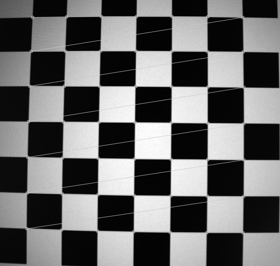
The image below shows an example output of the findChessboardCorners() function – OpenCV has successfully detected all internal corners of the distorted chess board image, which can subsequently be used to perform calibration.
The following code uses OpenCV’s calibrateCamera() function to determine the camera intrinsics matrix and distortion coefficients. The file storage API is used to persist the parameters to an XML file.
# calibrate camera: cameraMatrix = 3x3 camera intrinsics matrix; distCoeffs = 5x1 vector
# gray.shape[::-1] swaps single channel image values from h, w to w, h (numpy to OpenCV format)
retval, cameraMatrix, distCoeffs, rvecs, tvecs = cv2.calibrateCamera(objpoints, imgpoints, gray.shape[::-1], None, None)

# persist intrinsics and distortions
fs = cv2.FileStorage("intrinsics.xml", cv2.FileStorage_WRITE)
fs.write("image_width", gray.shape[1])
fs.write("image_height", gray.shape[0])
fs.write("camera_matrix", cameraMatrix)
fs.write("distortion_coefficients", distCoeffs)
fs.release()
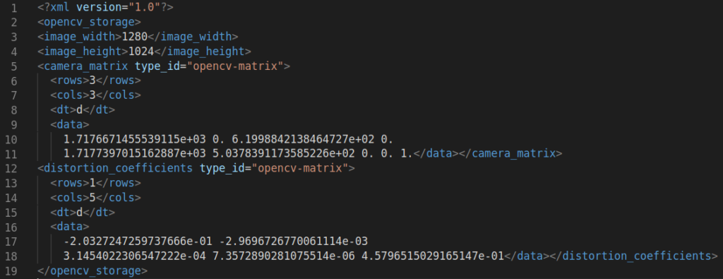
Upon inspection of the XML file in a text editor, we indeed have 4 values in the camera intrinsics matrix and 5 distortion coefficients.
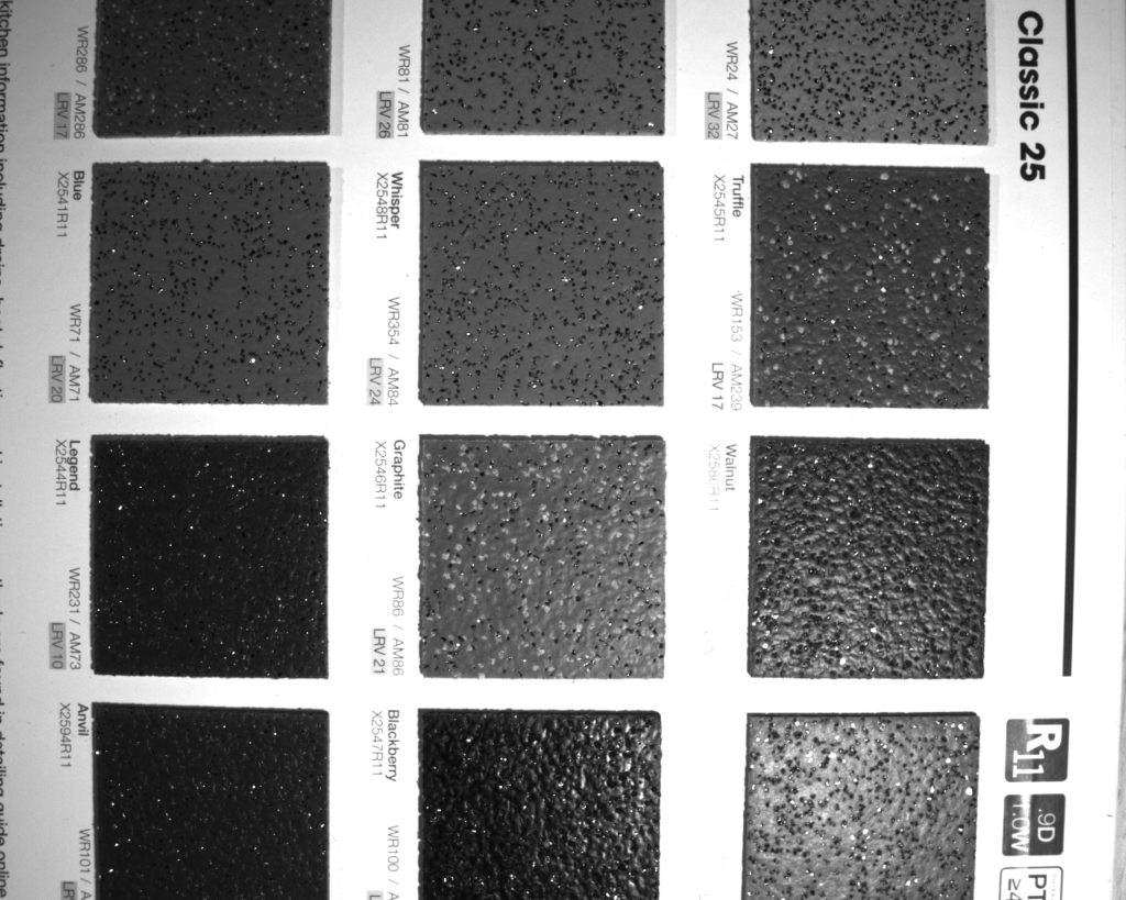
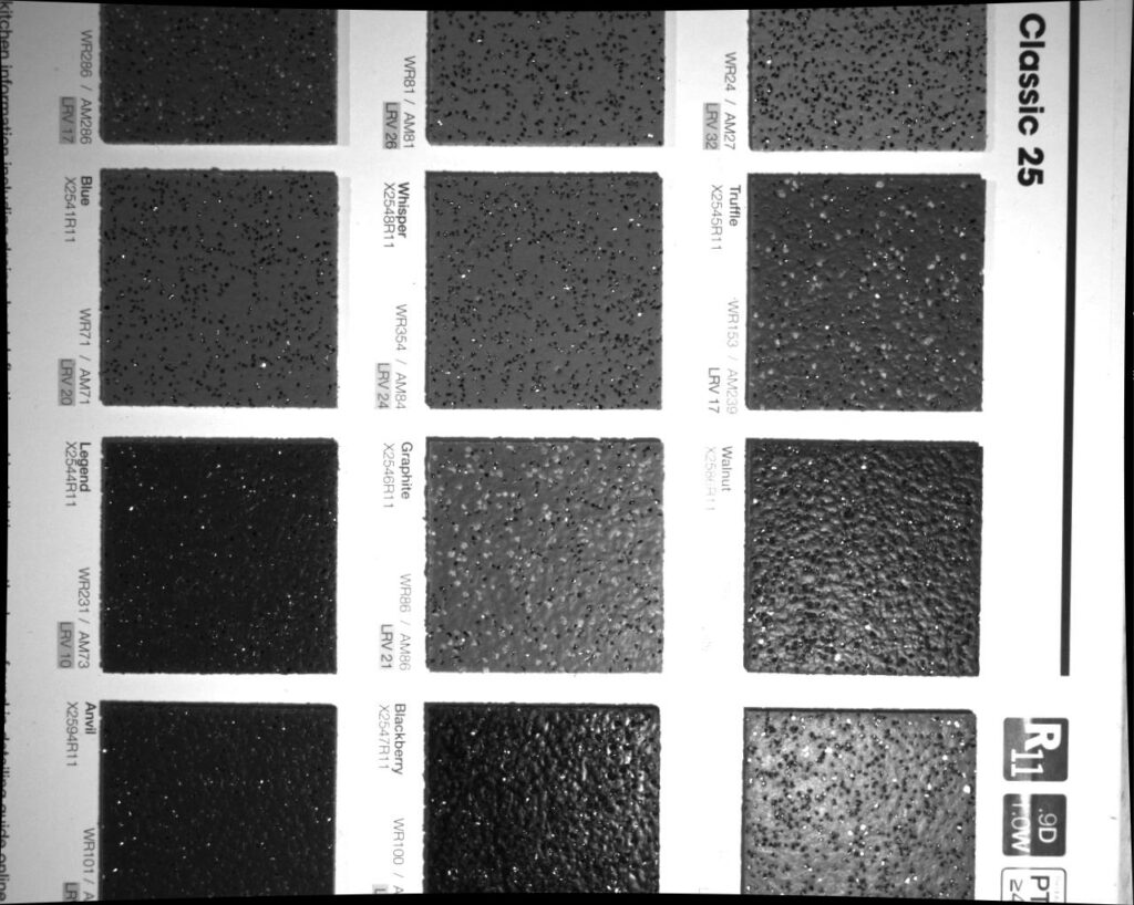
Having successfully obtained our parameters, we can import a new distorted image and apply OpenCV’s undistortion functions to straighten out the image. The image used is taken from a book of kitchen counter top samples which need to be processed for distortion prior to applying visual inspection functions – the barrel distortion is highly visible in the original image.
The following code refines the camera matrix for the image to be processed then computes and applies the transformations.
# input distorted image, leaving as 3 channel
image_dist = cv2.imread('./sample.png')
print("Distorted image shape: ", image_dist.shape)
cv2.imshow("Distorted Image", image_dist)
cv2.waitKey(0)

# refine camera matrix based on free scaling parameter and get valid ROI
h, w = image_dist.shape[:2]
cameraMatrixNew, roi = cv2.getOptimalNewCameraMatrix(cameraMatrix, distCoeffs, (w, h), 1, (w, h))

# compute undistortion and rectification transformation map
map1, map2 = cv2.initUndistortRectifyMap(cameraMatrix, distCoeffs, None, cameraMatrixNew, (w, h), cv2.CV_32FC1)

# apply undistortion and rectification maps to distorted 3 channel image
image_undist = cv2.remap(image_dist, map1, map2, cv2.INTER_LINEAR)
cv2.imshow("Undistorted Image Full", image_undist)
cv2.waitKey(0)
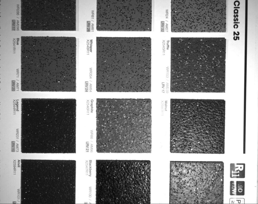
The image below is the undistorted output following transformation. The black patches at the edges are a by-product of the remapping process as the pixels are relocated for straightness.
Recognizing the black patches at the edges of the image above, OpenCV’s remapping functions provide a valid ROI (region of interest), giving the maximum rectangular image possible following transformation.
# crop undistorted image to valid ROI
print("Valid ROI: ", roi)
x, y, w, h = roi
image_undist = image_undist[y:y+h, x:x+w]
cv2.imshow("Undistorted Image Valid ROI", image_undist)
cv2.waitKey(0)
The resulting image is a cropped, valid ROI which can be subsequently be used as an input to visual inspection algorithms.
Conclusion
This article reviewed camera calibration theory at a high level, introducing the 9 parameters required to transform a distorted image (camera intrinsics matrix and distortion coefficients). A set of calibration chessboard images was used as an input to OpenCV’s calibration functions. The calibration parameters were calculated and saved to an XML file prior to being applied to a new distorted image.