
In Machine Learning literature, we often hear about the ‘model’ but what concretely is a Machine Learning model? This article explains the concept of data representation, which is central to the understanding of Machine Learning models.
As described in my previous blog article ‘Machine Learning: cut through the hype’, the underlying principle of Machine Learning is to automate the derivation of business rules using data and algorithms. In a supervised Machine Learning context, once a model is trained, its objective is to predict the output Ŷ given the input features X. The symbol Ŷ denotes that the output is a prediction rather than a real value of Y in the training data. The essence of the Machine Learning model is therefore a function, also known as a hypothesis, which maps input features X to a prediction Ŷ.
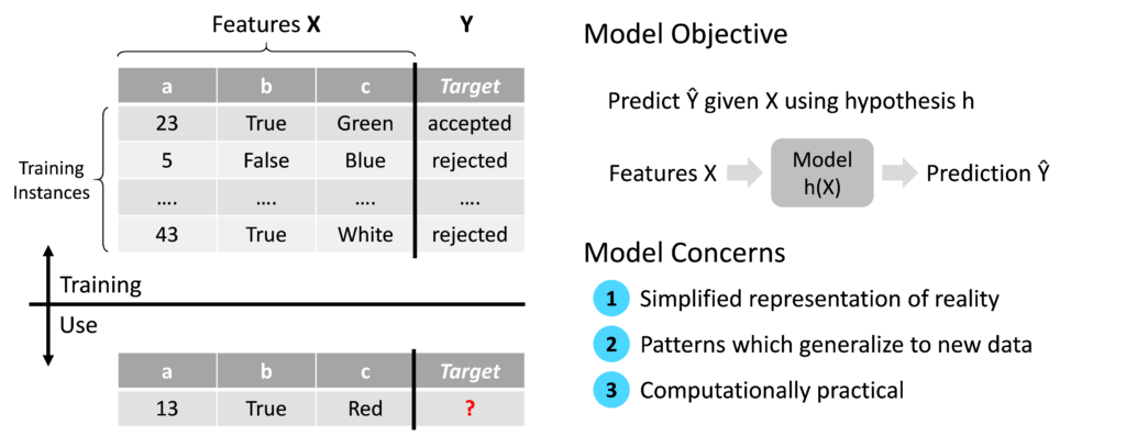
This objective considered, there are three key concerns regarding the design of a Machine Learning model:
Simplified representation of reality
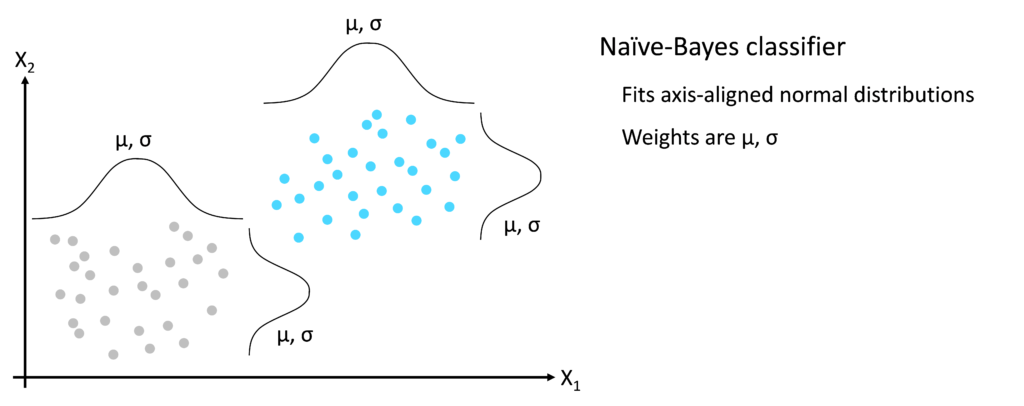
‘Reality’ refers to the training dataset i.e. real data collected for the purposes of building a model. The training dataset contains all of the raw details gathered during data collection, usually structured as a matrix of rows and columns. Each row is an individual training data instance. Each column is a feature, containing information captured for each data instance. In supervised Machine Learning, the final column of the training matrix is the target variable Y. The first concern of the model is to represent the training data matrix in a simplified form, based on the purpose of the model. For example, consider a supervised classification problem with two input features X1 and X2 – see image below. The target variable Y takes one of two values: grey or turquoise. The simplest form of Machine Learning classifier, Naive-Bayes, fits axis-aligned normal distributions to the clusters defined by the target variable Y. The simplified representation of reality therefore is the mean and standard deviation values of each of the normal distributions. The key point is that the model, a Naive-Bayes classifier in this case, takes a large number of training instances and represents them as a small number of normal distributions characterized by their mean and standard deviation values. The model therefore does not contain the raw training data but rather a simplified version of it, chosen based on the model’s purpose.
Patterns which generalize to new data
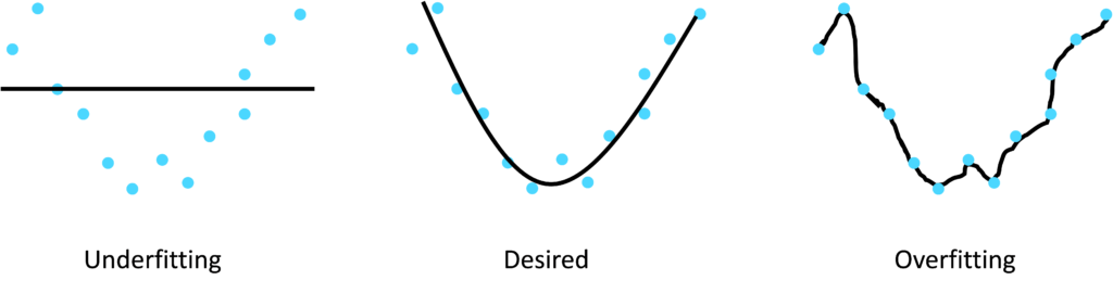
Training data typically contains two levels of patterns: those which generalize to new data and those which are specific to the training data. For example, consider a set of training data for a supervised regression problem to predict house prices. The columns of the training matrix are features characterizing the houses e.g. number of bedrooms, surface area, neighborhood etc. The target variable Y is the selling price of the house. The training data contains patterns which correlate the features X to the target Y i.e. linking house characteristics such as the number of bedrooms to the price of the house. Some of the patterns in the training set will be valid for houses beyond the training set i.e. patterns which generalize to new data instances which were not used to train the model. There will be a second level of patterns in the training data which do not generalize to new data instances i.e. they are specific to the particular houses represented in the training data. The second concern therefore of Machine Learning model design is to represent the patterns from the training data which do generalize to new data instances and ignore those which do not. ‘Overfitting’ refers to the situation where a model contains training data patterns which do not generalize to new data, thus reducing the ability of the model to make accurate predictions on new data instances.
Computationally practical
Inference refers to the action of introducing a new data instance to the model, for which we do not know the target variable Y, and executing the model to predict the target variable. Referring to the house price example introduced earlier in this article, once the model is trained, the price of a new house can be predicted by capturing the features of the new house and entering this into the model. Depending on the application, the acceptable time delay for completing the inference, i.e. predicting the new house price, can vary significantly. For example, a Machine Learning model used to perform voice recognition for smart phones needs to infer the answer in 2-3 seconds at most, otherwise it would be impractical for the smart phone user. Other applications do not have such demanding time constraints, for example a cancer tumor classifier could take several seconds or even minutes to infer the prediction and still be acceptable for the medical staff using the model. The third concern of the model design therefore is the maximum acceptable time delay within which the prediction needs to be computed. This time delay requirement can significantly influence the type of model chosen and the processing hardware on which the model runs.