
In the first of a series of blogs introducing the key Machine Learning models, we’ll start this week by looking at Linear Regression and how it can be applied to solve non-linear problems.
Linear data
The concept of a linear model is to make a prediction by calculating a weighted sum of the model’s input features, in addition to a constant which is often called the bias or intercept. A linear model in its simplest form is therefore a set of weights: one for each input feature plus the bias term. Let’s illustrate this using Scikit-Learn:
First we call the usual imports and set up the feature matrix X as a single column vector of 50 values equally spaced between 0 and 10. The model therefore has a single feature vector X. The target vector y is created from the X values using a bias term of 2, a weight of 1.5 and Gaussian noise from a random number generator.
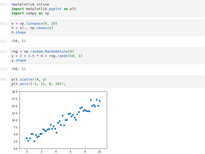
By instantiating Scikit-Learn’s LinearRegression class, we create a model, fit it to the training data and inspect the weights. The training process has generated weights close to those manually set above: a bias term of 2.85 and a feature weight of 1.36. To visualize the model, predictions are made using the original X values and plotted over the training data.
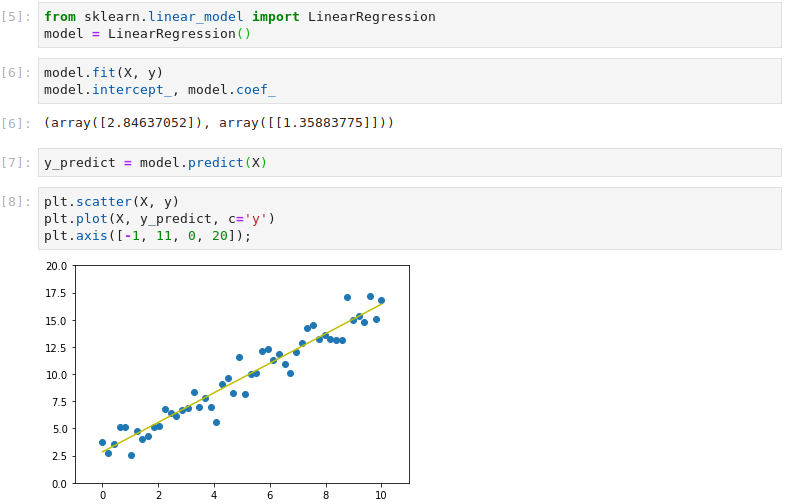
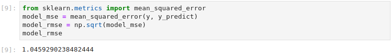
Scikit-Learn’s metrics library is used to calculate the Root Mean Square Error (RMSE), comparing the predicted target values with the training target values. This shows that, on average, the predictions are off by 1.05, which is to be expected given the Gaussian noise.
Non-linear data
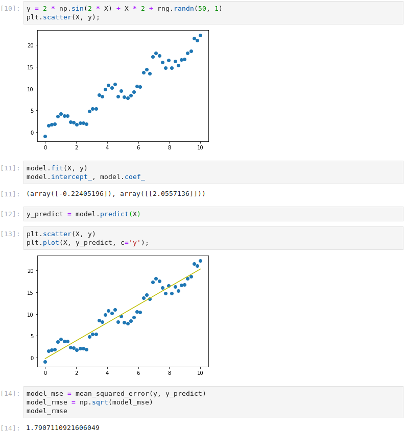
Let’s now explore how to tackle non-linear data. Firstly, we create a non-linear dataset by modifying a sine wave and adding random Gaussian noise. Clearly a straight line won’t fit this data very well. The Root Mean Square Error with a straight line fit is 1.79.
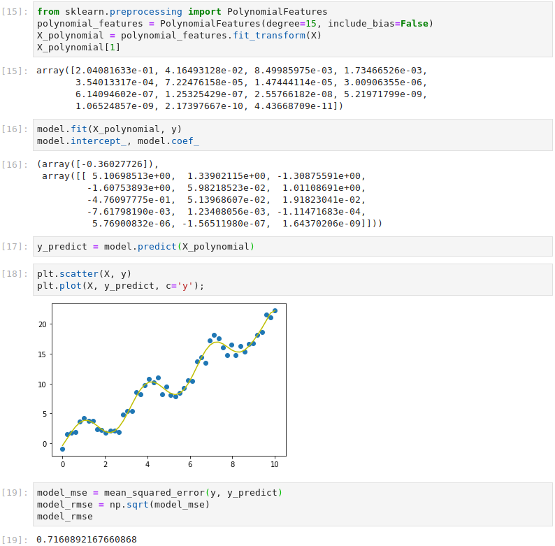
By applying Scikit-Learn’s PolynomialFeatures class, we can use a linear model to fit non-linear data. This transforms our training data by adding powers of the original feature X as new features i.e. X2, X3 etc. To allow a close fit, in this example we add new features up to the 15th degree polynomial (X15), adding 14 new features in total. By fitting the model to the expanded feature set and printing the weights, it can be seen that the model now has 15 feature weights and a bias term. The model remains linear as the weights never multiply or divide each other. By adding these extra features, the RMSE has been reduced to 0.72 without any new training data.
Conclusion
Linear Regression is the simplest of all Machine Learning models and, despite the more complex model types available, Linear Regression remains a useful tool for establishing an accuracy baseline before exploring more advanced techniques. This article has reviewed how linear models can fit non-linear data by transforming the training data with Scikit-Learn’s PolynomialFeatures class.