
Jupyter Notebooks are becoming the cornerstone tool for data scientists and Machine Learning practitioners. Why the sudden growth in popularity? This article reviews the history of Jupyter Notebooks and explains how to get started.
Background
Despite the recent surge in popularity, the concept of ‘computational notebooks’ started in 1988 with Wolfram Mathematica 1.0 on the Macintosh.
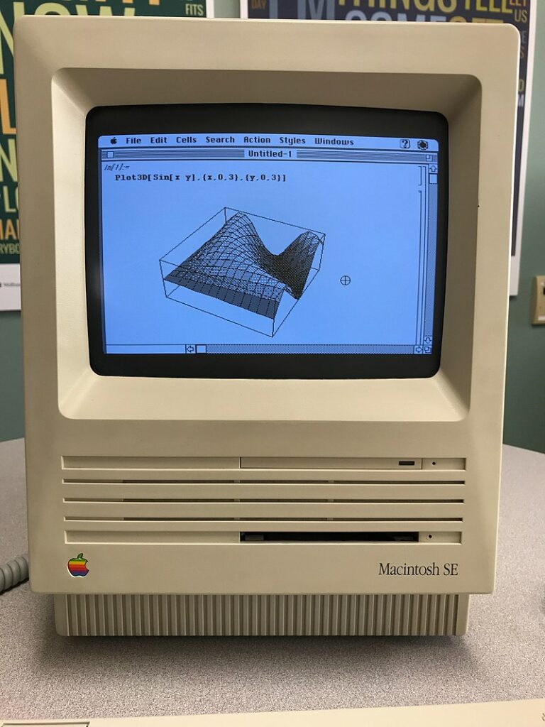
The idea is to combine word processing functionality with source code in a single interface, allowing supporting text, images and figures to be displayed inline with source code i.e. within the same notebook. The code portions of the notebook are contained within cells which can be executed individually or as a sequence.
This approach is considerably different to writing source code in text files which are executed as part of a program. For example, if the code above was written in a Python source file, the entire script would be executed on the command line or in an IDE and the plot would open in a separate window.
Project Jupyter came about recently when Fernando Perez spun the project off from IPython in 2014. IPython (Interactive Python) was started in 2001, providing a browser based computational notebook and an interactive shell for the Python language. Jupyter was launched to target more than just the Python language – the name reflects the core languages supported (Julia, Python and R). IPython still exists as the Python shell and default kernel for Jupyter but the notebook interface and language-agnostic parts of IPython were brought under the Jupyter umbrella.
Getting started
To begin with, we’ll need a virtual environment. For guidance on creating a virtual environment, see my previous blog post ‘Python basics: what is a virtual environment?’. Once the virtual environment is setup and activated, install Jupyter using the pip package manager.
$ python3 -m venv myenv
$ source ./myenv/bin/activate
(myenv) $ pip3 install jupyter
Having installed Jupyter, let’s introduce the concept of interactive computing by launching IPython in the shell. The command line screenshot below illustrates the essence of the IPython shell – it adds functionality beyond the standard Python interpreter to provide a more interactive experience. For example, IPython’s In / Out variables and ‘?’ help commands provide the interactive feel which has popularized Jupyter Notebooks. A full list of IPython commands can be found on the IPython website.
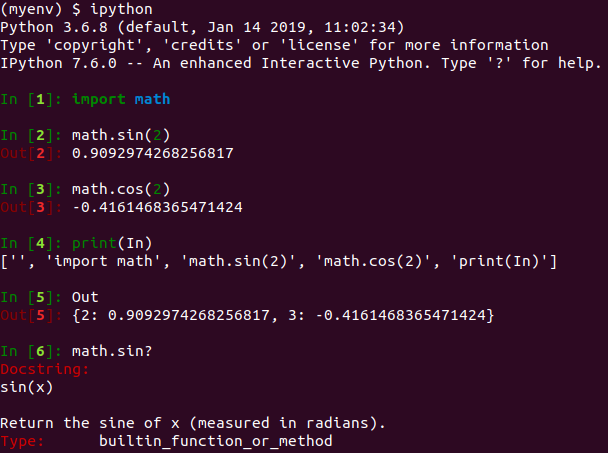
The IPython shell remains a useful tool for testing out short stubs of code but the real power of the computational notebook is apparent when it’s used in the browser. The following command launches the Jupyter Notebook server and opens a browser page displaying the Jupyter dashboard.
(myenv) $ jupyter notebook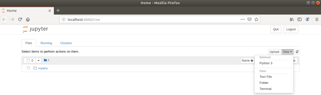
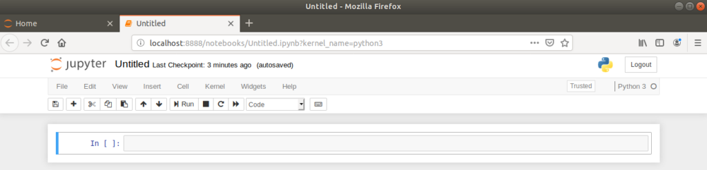
Clicking on ‘New > Python 3’ creates a new, untitled notebook which is opened in a new browser tab.
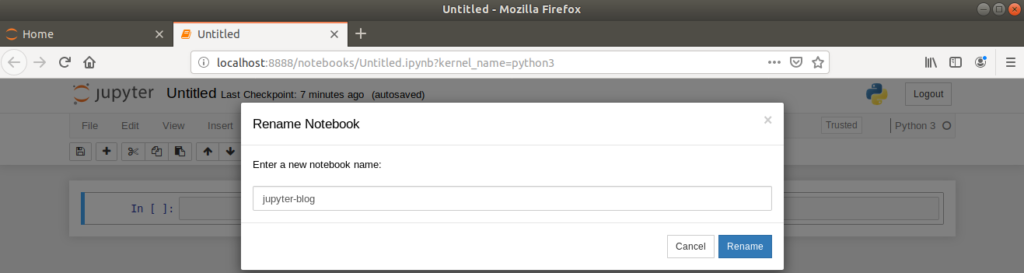
It’s important to rename the notebook to something appropriate for future use. This is done by clicking on the ‘Untitled’ text, which opens a dialog box for renaming.
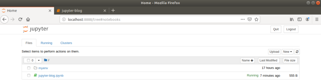
Returning to the dashboard browser tab will now show the new, renamed notebook saved as a .ipynb file.
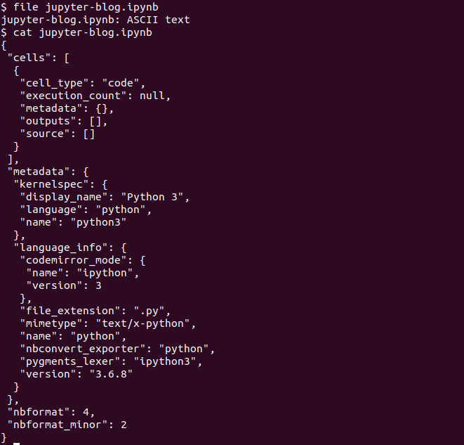
As additional background information, the .ipynb file extension comes from the term ‘IPython Notebook’, reflecting Jupyter’s origins. These files are ASCII text files with JSON content.
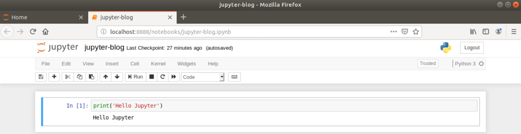
Returning to our newly created Jupyter Notebook, each line of the notebook is called a ‘cell’, which by default is set to receive Python code. When code is entered into a cell, the cell is ran by clicking the ‘Run’ button or by typing Ctrl+Enter.
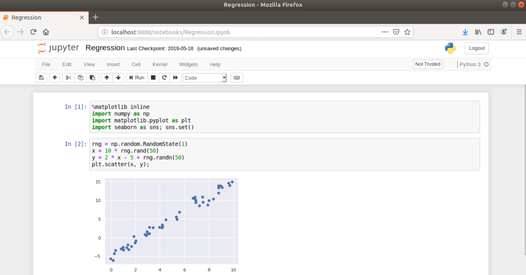
Let’s illustrate the inline plotting functionality by drawing a sine wave. First, returning to the command line, we’ll install the numpy and matplotlib packages in our virtual environment.
(myenv) $ pip3 install numpy matplotlibHaving successfully installed the necessary packages, we can import the required functions into our notebook in order to draw a sine wave.
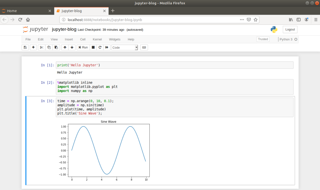
This simple example illustrates the inline nature of Jupyter Notebooks, which is particularly useful when developing Machine Learning models as plots can easily be viewed, saved and re-plotted alongside the source code.
JupyterLab
In February 2018, Project Jupyter announced their latest product – JupyterLab. This is an evolution of the Jupyter Notebook which provides additional functionality such as built-in code editors, terminals and file system viewers. JupyterLab is installed as a separate package, which is fully compatible with Jupyter Notebook .ipynb files.
(myenv) $ pip3 install jupyterlab
(myenv) $ jupyter lab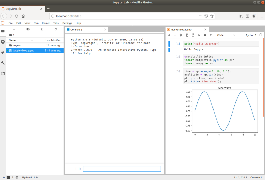
Conclusion
Taking a very different approach to a traditional IDE, Jupyter Notebooks and their successor JupyterLab have quickly become the ‘go to’ tools for Data Scientists and Machine Learning practitioners. They are particularly useful when displaying figures inline with code and running small segments of code is desired, which is often the case in Machine Learning model development.