Machine Learning models are ‘trained’ but what concretely does ‘training’ mean in the context of a model? This article explains the model training process and the elements of the model training loop.
As described my previous blog post ‘Machine Learning basics: what is a model?’, the overall objective of the model in a supervised Machine Learning context is to predict the output Ŷ given the input features X. The symbol Ŷ denotes that the output is a prediction rather than a real value of Y in the training data. The key concern of the model design is to provide a simplified representation of reality which generalizes to new data and is computationally practical.
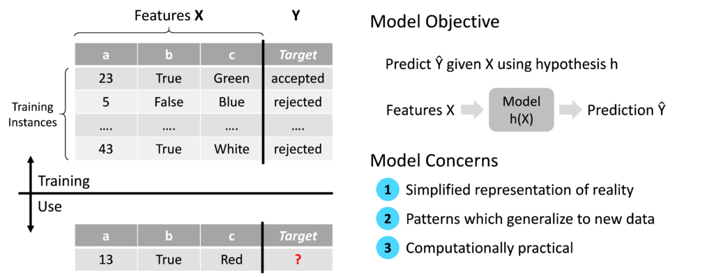
‘Training’ refers to the creation of the model from the training data. More specifically, the objective of the model training process is to optimize the model’s weights in order to achieve an acceptable level of prediction accuracy without overfitting the training dataset. The training process consists of three elements: the model, the loss function and the optimizer.
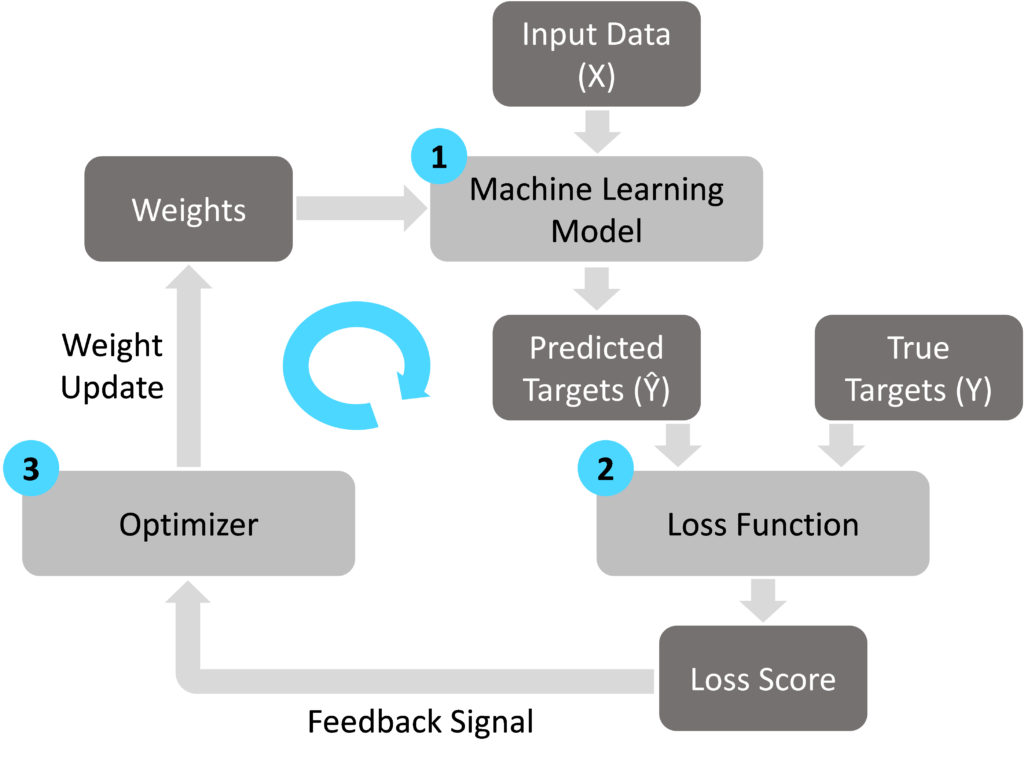
Element one, the model, is the output of the training process which is deployed into a production scenario when a sufficient level of maturity is achieved. For more information on the model objectives and design, see my previous blog post ‘Machine Learning basics: what is a model?’.
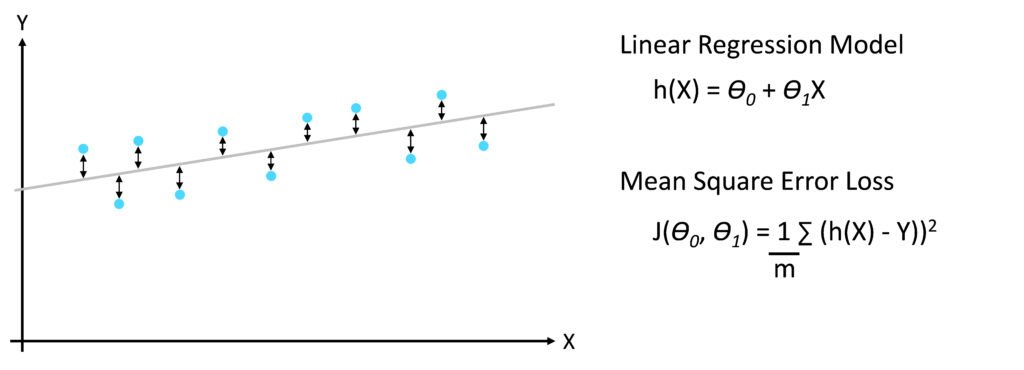
Element two, the loss function, compares the predictions made by the model (Ŷ) to the actual target values in the training dataset (Y). The objective of the loss function is to represent the difference between the predicted values Ŷ and the true targets Y as a single number, the loss score. The loss function is also known as the ‘cost function’. As a simple example, a supervised linear regression problem with a single input feature X uses two weights (Ɵ0 and Ɵ1) to predict the target value Y. There are various methods of calculating the loss score J. A common approach is to take the mean of the squared distances between the predicted and actual target values.
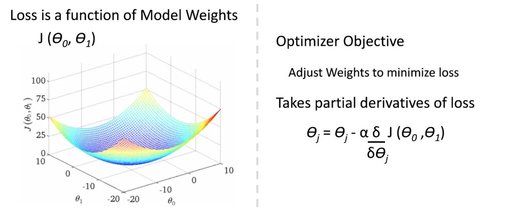
The loss score is fed into element three, the optimizer, which uses the loss score to optimize the model weights. The goal of the optimizer is to improve the model’s accuracy without overfitting the training dataset. Building on the linear regression example above, the loss score can be plotted as a function of the model weights (Ɵ0 and Ɵ1), giving a three-dimensional plot in this case. Given a set of initial model weights, the optimizer works its way down the loss function curve to seek the model weight values which give the lowest possible loss score. Mathematically, optimizers typically take partial derivatives of the loss function to determine the direction in which the model weights should be adjusted.
The model training loop is ran on an iterative basis to gradually move towards the optimum model weights. Depending on the type of model used, the number of training iterations can be a factor in model overfitting as each iteration of the training loop fits the model closer to the training dataset.
