
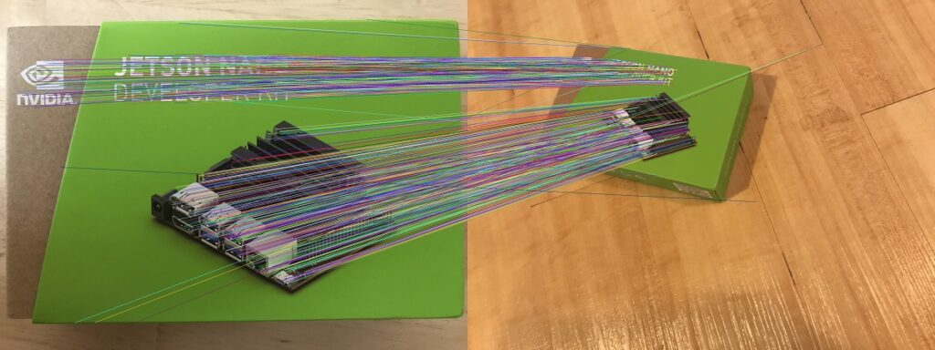
Keypoint detection and matching remains a cornerstone of object detection despite the more recent introduction of Deep Learning based approaches. Keypoint detection shows impressive invariance to translation, scaling, rotation, lighting and 3D projection, allowing powerful object detectors to be created. The image below illustrates what can be achieved with keypoint detection and matching – keypoints are matched despite considerable differences in scale, rotation and 3D projection. The purpose of this article is to explain how such invariance is achieved.
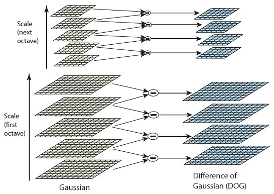
There are many types of keypoint detectors and extractors. For the purpose of this article, we’ll focus on the Difference of Gaussian keypoint detector, which is part of the well-known SIFT technique (Scale Invariant Feature Transform). The first stage of processing is to generate what are known as ‘scale space’ images. For a given image, progressively blurred versions are created using Gaussian filters, resulting in an ‘octave’. The original image is then halved in size and another octave is created by once again generating progressively blurred versions. This progressive scaling and blurring is the key to achieving invariance.
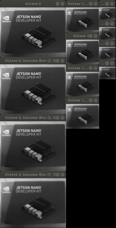
Having created octaves at various scales, we create a ‘Difference of Gaussian’ for each consecutive pair of blurred images in a given octave. The next blurred image in the octave is simply subtracted from the previous one. This results in a series of Difference of Gaussian images for each octave (scale) of the original image.
The image below demonstrates the Difference of Gaussian operation, subtracting the 5×5 Gaussian Blur from the 3×3 Gaussian Blur.

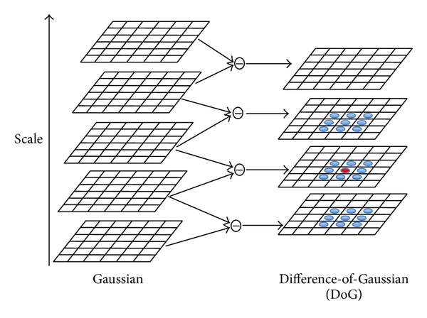
Once the Difference of Gaussian images are generated for each octave (scale), keypoints are identified by comparing each Difference of Gaussian pixel to its 8 surrounding pixels and to the 9 corresponding pixels in the Difference of Gaussian layer above and below, giving 26 comparisons in total. Pixels are considered keypoints if they have an intensity level greater than or less than all 26 comparison pixels.
The technique of progressively blurring at various levels of scale gives the keypoint detection technique its invariance to translation, scaling, rotation, lighting and 3D projection. The size of the circles in the image below indicates the scale at which each keypoint was identified.

Having identified keypoints, a feature extractor can be used to generate a vector describing the area surrounding the keypoint. As described in a previous blog post, the resulting feature vectors can then be matched between different images using Machine Learning techniques.