
One of the key aims of image processing is the demarcation of objects in digital images. This process is called image segmentation, which thresholding provides a simple means of achieving. This article uses OpenCV to demonstrate how objects can be segmented using simple thresholds. Automatic and Adaptive Thresholding techniques are explained for handling varying lighting and reflective conditions.
Global Thresholding
The basic idea of thresholding is that something happens to every element of the image depending on whether it is above or below the threshold. This can be viewed as a simple convolution operation that uses a 1 x 1 pixel kernel and performs a non-linear operation on each individual pixel. A simple binary threshold sets each pixel to a high or low value.
Global Thresholding refers to a single threshold value being applied over the whole image. To demonstrate this with OpenCV, we first import the OpenCV Python bindings and Matplotlib, followed by a read and presentation of a grayscale image showing a wrench on a workbench.
import cv2
from matplotlib import pyplot as plt

wrench = cv2.imread("wrench.png", cv2.IMREAD_GRAYSCALE)
cv2.imshow("Wrench", wrench)
cv2.waitKey(0)

In order to determine the threshold value, it’s useful to see a histogram of the pixel values. The following Matplotlib code displays pixel values on the x-axis and pixel count on the y-axis.
plt.hist(wrench.ravel(),256,[0,256]); plt.show()
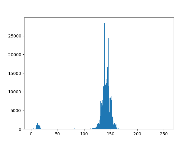
The histogram above clearly shows two peaks: the peak on the left representing the darker pixels of the wrench and the peak on the right representing the workbench surface. A threshold value of 50 should segment the image nicely. The following code uses OpenCV’s threshold() function to apply a binary threshold of 50 and present the resulting image.
(T, wrench_50) = cv2.threshold(wrench, 50, 255, cv2.THRESH_BINARY)
cv2.imshow("Wrench Threshold 50", wrench_50)
cv2.waitKey(0)
The darker areas of the wrench are well segmented however the polished steel surfaces are grouped with the workbench surface, which could be corrected by fine-tuning the threshold.

Automatic Global Thresholding
Manually setting a fixed global threshold as in the previous section has limitations when lighting conditions change. The code below reads and presents the same image scenario with a higher level of white light illumination.
wrench_illum = cv2.imread("wrench_illumination.png", cv2.IMREAD_GRAYSCALE)
cv2.imshow("Wrench Illumination", wrench_illum)
cv2.waitKey(0)

By inspecting the histogram, it can be seen that the peaks are still visible however they have moved to the right as a result of the increased illumination.
plt.hist(wrench_illum.ravel(),256,[0,256]); plt.show()
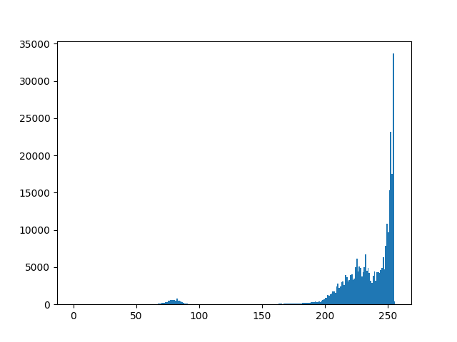
Our threshold value of 50 clearly wouldn’t work in this increased illumination scenario. This highlights how slight changes in background lighting can easily affect thresholding. A solution to this is to automatically recalculate the threshold image-by-image to achieve optimum segmentation. Otsu’s algorithm considers all possible thresholds and minimizes the variance for each of the two classes of pixels (the class above the threshold and the class below it), automatically setting the global threshold. The code below applies Otsu’s algorithm to perform binary thresholding on the wrench image with higher illumination.
(T, wrench_illum_otsu) = cv2.threshold(wrench_illum, 0, 255, cv2.THRESH_BINARY | cv2.THRESH_OTSU)
cv2.imshow("Wrench Illumination Otsu", wrench_illum_otsu)
print("Otsu's threshold: {}".format(T))
cv2.waitKey(0)
Otsu’s algorithm automatically picked a threshold of 160, which segments the image almost as effectively as the manual value picked in the previous section.

Adaptive Thresholding
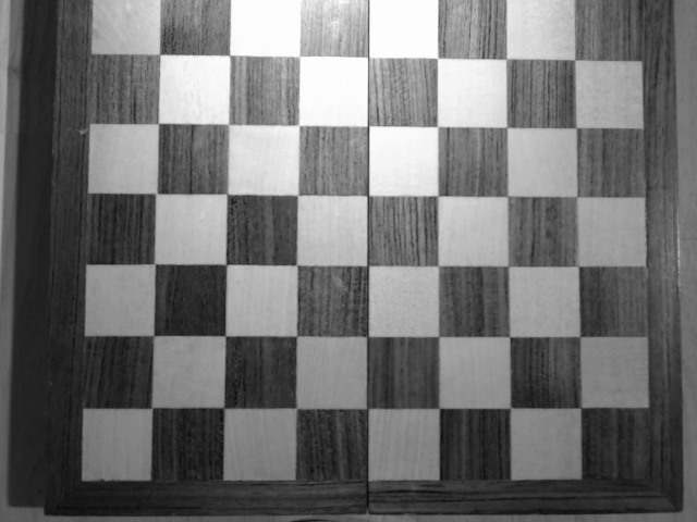
Otsu’s algorithm is useful for handling changes in background lighting which equally affect pixel intensity across the whole image. Where global thresholds run into difficulty is the presence of strong illumination or reflectance gradients across the image. The following grayscale image of a chess board has higher illumination in the upper-center area and dark regions in the lower corners.
chess = cv2.imread("chess.png", cv2.IMREAD_GRAYSCALE)
cv2.imshow("Chess", chess)
cv2.waitKey(0)
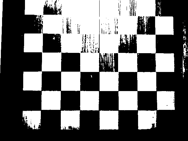
The code and image below demonstrate that a global threshold, even when calculated using Otsu’s algorithm, struggles to segment an image with illumination gradients.
(T, chess_otsu) = cv2.threshold(chess, 0, 255, cv2.THRESH_BINARY | cv2.THRESH_OTSU)
cv2.imshow("Chess Otsu", chess_otsu)
cv2.waitKey(0)
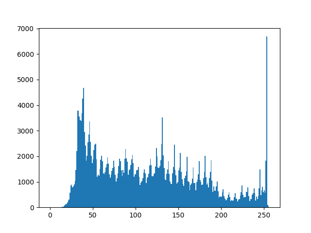
Upon inspection of the histogram, it can be seen why a global threshold fails to effectively segment the image. There is no single clear valley in the histogram in which a global threshold could be placed.
plt.hist(chess.ravel(),256,[0,256]); plt.show()
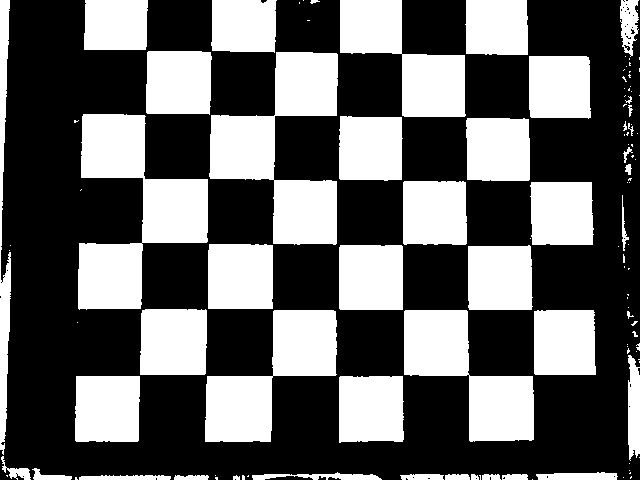
Adaptive Thresholding modifies the threshold locally across the image, rather than thresholding on a single global value. The adaptive threshold is computed on a pixel-by-pixel basis by calculating a weighted average of the region around the pixel, minus a constant. The code below uses a 101 x 101 region with a constant of -15 to apply an adaptive binary threshold. The results are positive, with clean segmentation reaching into all regions of the image.
chess_adaptive = cv2.adaptiveThreshold(chess, 255, cv2.ADAPTIVE_THRESH_MEAN_C, cv2.THRESH_BINARY, 101, -15)
cv2.imshow("Chess Adaptive", chess_adaptive)
cv2.waitKey(0)
Conclusion
Thresholding is a simple means of achieving image segmentation. A global threshold can be used, which can be made more intelligent by applying Otsu’s algorithm to handle changes in background lighting. Where strong illumination or reflectance gradients are present, adaptive thresholding can be applied to account for pixel intensity changes across the image.